Key rate durations and convexities measure your portfolio’s risk towards changes in specific key interest rates. But when do the individual durations and convexities add up to your overall measures based on parallel shifts? And how well do the delta and gamma vectors represent the nature of the underlying bonds? We have done the math and provide you with some (surprising?) answers and further insight on this topic.
Duration and convexity are classical measures of a bond’s price sensitivity to a parallel shift in interest rates, and as such they are fundamental inputs to the management of risks in your portfolio. However, they do not provide you with information on the risks associated with real-life, non-parallel shifts in the yield curve.
Key rate durations and convexities are one way you can measure expected bond price changes resulting from arbitrary yield curve shifts. In 1992, Thomas Ho1 introduced key rate durations as the price sensitivity to changes in key rates of specific maturities, obtained by applying a series of triangular shifts to the spot rate at the key maturity points. The triangular shifts are constructed such that they sum to a parallel shift of the yield curve. Figure 1 shows a set of triangular spot rate shifts.
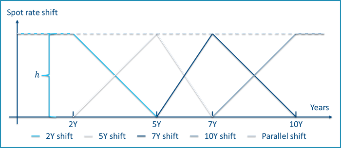
Figure 1 - Triangular spot rate shifts of size h defined by maturity points 2Y, 5Y. 7Y, and 10Y.
The key rate measures lead to several interesting questions, many of which we are also often asked by our clients, and we will answer two of the most common in this blog:
- The yield curve shifts underlying the key rate measures sum exactly to a parallel shift, but under which circumstances do the key rate durations/convexities sum exactly to the duration/convexity?
- Do the vectors of sensitivities show a reasonable distribution on the key rate maturities relative to the nature of the bond in question?
If you are interested in a deeper analysis, please see our 2018 Scanrate Model Service white paper on the subject available for Scanrate Model Service subscribers at Scanrate Model Service
Calculating key rate duration and convexity
In order to calculate key rate risk measures, we need to apply discretizations of the duration and convexities as there are generally no closed form solutions.2 Using approximations inevitably introduces a discretization error, which may differ in size and sign depending on the method used. A small error leads to a high precision of the approximation.
Figure 2 illustrates how duration and convexity measures are found and interpreted based on the price-yield relationship for the typical case of a non-callable bond with positive convexity. The dollar duration approximates the slope of the price-yield curve, whereas the dollar convexity approximates the change in slope, i.e. the curvature.
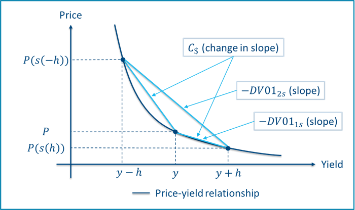
Figure 2 - Discretized dollar duration and convexity based on a positive convex price-yield relationship. Two shifts, \(s(h)\) and \(s(-h)\), are applied to spot rates to obtain the shifted prices.
For those of you who are into formulas, we present those as well. If \(s\) denotes some shift to the yield curve, \(h\) is the shift size, and \(P(s(h))\) is the price of the bond obtained from the shifted yield curve, the one-sided (“1s”) dollar duration measure found using an upward shift is:
$$DV01_{1s}=-\frac{P(s(h))-P}{h}$$
Increased precision may be obtained by applying a two-sided shift (“2s”) where the yield curve is shifted both up- and downwards using the same shift:
$$DV01_{2s}=-\frac{P(s(h))-P(s(-h))}{2\cdot h}$$
The dollar convexity measure is always two-sided and defined as:
$$C_{$}=\frac{P(s(h))-2\cdot P+P(s(-h))}{h^2}=\frac{\frac{P(s(h))-P}{h}-\frac{P-P(s(-h))}{h}}{h}$$
When the shift \(s\) is parallel, the above formulas give rise to the duration and convexity, whereas the individual key rate durations/convexities are found when \(s\) is a triangular (or similar) shift.
Designing shifts that add up
Key rate measures based on triangular shifts do not always sum to the corresponding parallel measures as shown further below. However, it is possible to define a set of shifts that possesses this quality. We denote these left- and right-adjusted shifts and present them below.
The basic idea is to “set out” with the unshifted curve, and then “move through” the key rate maturities using a set of shifts that gradually shifts an increasingly larger portion of the yield curve, finally “ending up” in the full parallel shift at the last key rate. For left-adjusted shifts, the outset is to the left, i.e. the movement is from the smallest to the largest key rate maturity, whereas right-adjusted shifts have outset to the right at the largest key rate maturity moving left towards the smallest maturity.
The shifts are designed such that the difference between two consecutive shifts is the corresponding triangular shift. Therefore, each key rate figure is defined using the price difference from the two consecutive shifts surrounding its maturity. Intuitively, the resulting key rate measures add up because the intermediate prices cancel out, leaving only the difference between the start and end prices based on a zero shift and the full parallel shift.
Figure 3 shows an example of left- and right-adjusted shifts used to calculate the 5Y key rate figures. The shifts are named after the key rate maturity at which the shift breaks of from a parallel movement to a linear decline.
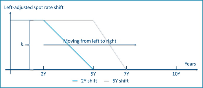
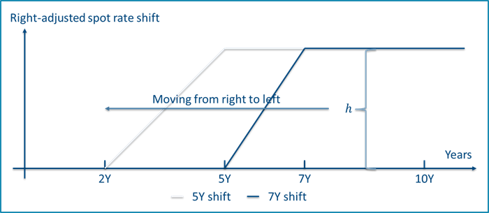
Figure 3 - Left-adjusted spot rate shifts (top) and right-adjusted shifts (bottom) used to calculate key rate figures at 5Y maturity. The full set of shifts are defined by maturity points 2Y, 5Y, 7Y and 10Y and a shift size $h$.
For the mathematically minded, we provide the key rate duration formulas using right-adjusted shifts as an example3. To ease notation, let \(P^h_i=P(s^r_i(h))\) where \(s^r_i\) is the i’th right adjusted shift at key rate maturity point \(i\):
$$DV01_{1s,i}=-\frac{P^h_i-P^h_{i+1}}{h}$$
for the single-sided case, and for the two-sided case:
$$DV01_{2s,i}=-\frac{(P^h_i-P^h_{i+1})-(P_{i}^{-h}-P^{-h}_{i+1})}{2 \cdot h}$$
where we define \(P(s_{N+1}(h))=P\), as we start out from the right using the unshifted curve. The right-adjusted key rate convexities are defined as:
$$C_{\$,i}=\frac{(P^h_i-P^h_{i+1})-(P^{-h}_{i+1}-P^{-h}_{i})}{h^2}$$
|
Fact box - Adding up left- and right-adjusted key rate measures The key rate measures based on left- or right-adjusted shifts add to the corresponding parallel measure by construction. Consider the right-adjusted, one-sided key rate durations: $$\displaystyle\sum_{i=1}^{N}DV01_{1s_i}=-\frac{1}{h}\displaystyle\sum_{i=1}^{N}(P^h_i-P^h_{i+1})=-\frac{1}{h}(P^h_1-P^h_{N+1})=-\frac{P_p-P}{h}=DV01_{1s}$$ The first equality follows from the key rate duration definition, the second equality follows as the sum is telescoping and therefore cancels out all intermediate prices. The third equality follows because a set of right-adjusted shifts starts from the right with a unshifted curve and ends to the left with the fully shifted curve. The final equality is the very definition of the (discretized) dollar duration. Similar arguments apply for left-adjusted shifts, where the first shift from the left is the unshifted curve and the last shift to the right is the parallel one. The arguments also extend to the case of two-sided duration and convexity.
|
When do key rate measures add up?
Based on a set of key rates placed in maturities 1Y, 2Y, 5Y, 7Y, 10Y, 20Y and 30Y we compare the dollar duration and convexity to the sum of key rate dollar durations and convexities. The instrument is a Danish 4.5%-2039 non-callable government bond with a bullet profile (DK0009922320), and the results are presented in Table 1.
| KEY RATE SHIFT | \(DV01_{1s}\) | $$\displaystyle\sum_{i}DV01_{1s,i}$$ | \(DV01_{2s}\) | $$\displaystyle\sum_{i}DV01_{2s,i}$$ | $$C_\$$$ | $$\displaystyle\sum_{i}C_{\$,i}$$ |
|---|---|---|---|---|---|---|
| Triangular | 24.9549 | 25.0268 | 25.2038 | 25.2030 | 4.9782 | 3.5242 |
| Left-adjusted | 24.9549 | 24.9549 | 25.2038 | 25.2038 | 4.9782 | 4.9782 |
| Right-adjusted | 24.9549 | 24.9549 | 25.2038 | 25.2038 | 4.9782 | 4.9782 |
| Average of left- and right-adjusted | 24.9549 | 24.9549 | 25.2038 | 25.2038 | 4.9782 | 4.9782 |
Table 1 - Comparison of dollar duration and convexity to sum of key rate dollar and convexity, respectively. Key rate maturities are 1Y, 2Y, 5Y, 7Y, 10Y, 20Y and 30Y. The instrument is a Danish 4.5%-2039 non-callable government bullet bond. Differences are marked with bold. Numbers are calculated on 15 February 2018.
We have done the math, and we found that the results are completely general for non-callable bonds. The main takeaways are therefore:
|
Key results when adding key rate durations and convexities
|
It’s all about convexity
We learned from the above example that key rate durations do not add up to the duration when using triangular shifts, even for a bond with no embedded optionality. This is because of the convexity in the price-yield relationship of the bond.
We illustrate this using a single-sided shift and a zero-coupon bond with a maturity somewhere between 5 and 7 years from today. Figure 4 shows the parallel shift as well as the two relevant key rate shifts surrounding the single bond payment at maturity.
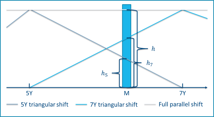
Figure 4 - A parallel shift of size h as well as the 5Y and 7Y triangular shifts relevant for the calculation of (partial) durations for a zero-coupon bond maturing at time M between 5 and 7 years from today.
It is seen that the triangular yield curve shifts add up to the size of the parallel shift at the bond maturity as \(h_5+h_7=h\). However, a similar equality does not hold in prices because of the convexity in the price-yield relationship.
In Figure 5, the zero-coupon bond example is illustrated using price-yield relationships. The price-yield relationship inherits a convex nature from the yield curve’s discount function. We observe that the bond price changes by \(\Delta P_P\) when the yield is increased from \(y^*\) to \(y^*+h\). By the definition above, the parallel dollar duration reflects this price change in a single step represented by the straight, light blue line.
The partial durations split the single yield change into two steps both originating in \(y^*\). The price changes by \(\Delta P_5\) when applying the 5 year triangular shift, and the 7 year triangular shift results in price change of \(\Delta P_7\). It is clear from the graphical illustration that the sum of these two price changes is larger than the price change from the parallel shift \(\Delta P_P\). Mathematically, this is due to the convexity of the price-yield relationship obeying to Jensen’s inequality. As an end result, the key rate dollar durations do not sum to the dollar duration, and we overestimate the actual price change when summing one-sided partial durations under positive convexity.
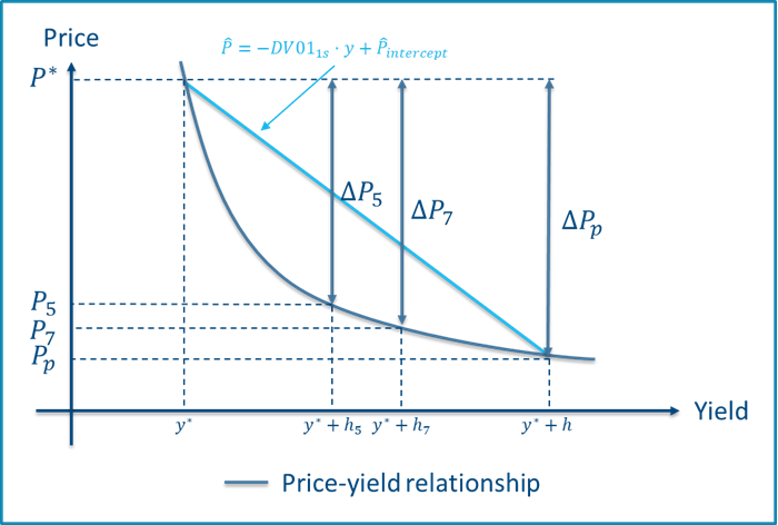
Figure 5 - Price-yield relationship of zero-coupon bond including price changes obtained from a full parallel shift, \(\Delta P_P\), as well as price changes from triangular shifts at 5Y and 7Y, \(\Delta P_5\) and \(\Delta P_7\), respectively.
Some concluding remarks:
- The example covers a zero-coupon bond, that is a single payment. However, a non-callable bond may be seen as a series of zero-coupon bonds, and therefore the arguments extend to non-callable bonds in general. No offsetting is possible because the convexity is strictly positive without embedded options
- The sum of one-sided durations overestimates the duration. It can be shown that the sum of two-sided key rate durations underestimates the overall duration, but with a better precision
- The convexity in the example is exaggerated to emphasize the main points. In reality, effects on durations are much smaller as seen from the calculations in Table 1
- Adding optionality such as prepayment options complicates things further as the convexity may become negative at some interest rate levels. However, the main conclusion remains – key rate measures based on triangular spot rate shifts do not generally sum to the corresponding parallel measure, but based on left- or right-adjusted shifts they do!
Left or right? Use the average!
Using left- or right-adjusted shifts is the way to go if you want your key rate measures to add to the corresponding parallel measures. However, the choice between the two shift types has a significant impact on how the total risk is distributed on the individual key rates, especially for convexities. To provide a useful solution to this problem, we introduce a simple average method. As indicated by the name, the average method is just the average of the left- and right-adjusted key rate measures:
$$DV01^a_{1s,i}=\frac{1}{2}\cdot [DV01^l_{1s,i}+DV01^r_{1s,i}]$$
$$DV01^a_{2s,i}=\frac{1}{2}\cdot [DV01^l_{2s,i}+DV01^r_{2s,i}]$$
$$C^a_{\$,i}=\frac{1}{2}\cdot [C^l_{\$,i}+C^r_{\$,i}]$$
where superscripts \(a\), \(l\) and \(r\) corresponds to average, left and right, respectively. As both the left- and right-adjusted measures add up to the corresponding parallel measure, this is also trivially the case for the average method.
Delta vectors
We set out by illustrating the delta vectors, i.e. key rate dollar durations. We consider the one-sided case for the Danish 4.5%-2039 non-callable government bullet bond (DK0009922320). We use a rather large shift size of 100 bps to emphasize our conclusions. The delta vectors based on all four methods are shown in Figure 6.
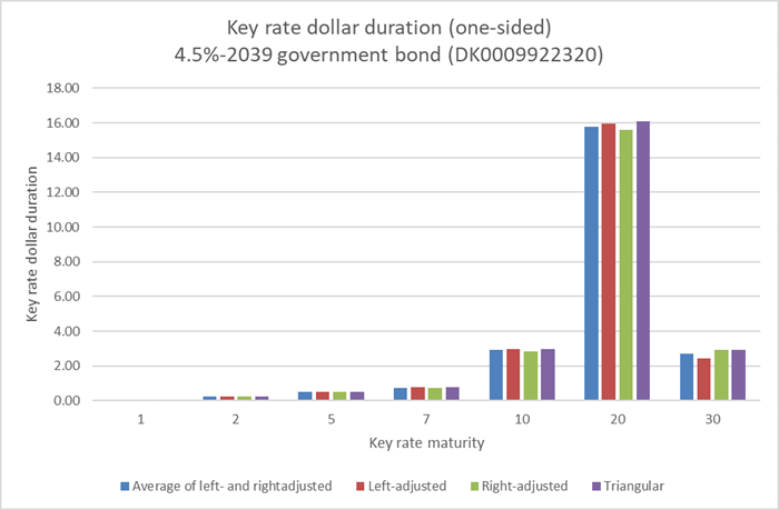
Figure 6 - One-sided key rate dollar durations for the Danish 4.5%-2039 non-callable government bullet bond (DK0009922320) based on a shift size of h=100 bps. The calculation date is 15 february 2018, i.e. the bullet bond has 21 years to maturity.
The bullet bond pays a fixed coupon of 4.5% per year and is non-callable with 21 years to maturity, and we therefore expect the durations to be centered around the 20 year key rate which is also the case. Furthermore, we observe that the triangular shifts give rise to the largest key rate durations for all maturities. This is in line with our previous finding that one-sided triangular spot rate shifts result in too much duration.
The large payment at maturity is distributed differently on the 20Y and 30Y key rates by the left- and right-adjusted methods. The left-adjust shifts attribute more duration to the 20Y key rate relative to the 30Y key rate when compared to the right-adjust method. This observation exemplifies the main difference between key rate durations based on left- and right-adjusted shifts.
Again, we have done the math and present you with the general results to remember:
|
Key results for key rate durations
|
Gamma vectors and the convexity push
We continue our illustrations using gamma vectors, i.e. key rate dollar convexities. These are shown in Figure 7 for the 4.5%-2039 government bond using a shift size of 10 bps.
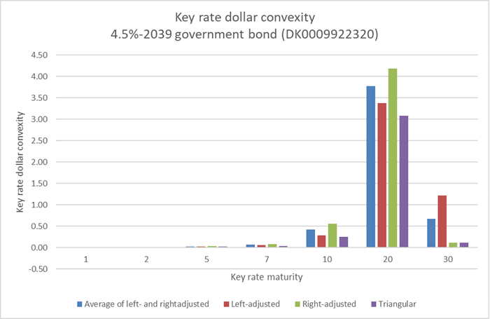
Figure 7 - Key rate dollar convexities for the Danish 4.5%-2039 non-callable government bullet bond (DK0009922320) based on a shift size of h=10 bps. The calculation date is 15 february 2018, i.e. the bullet bond has 21 years to maturity.
From the example, it is seen that the key rate dollar convexities based on triangular shifts are generally lower compared to left- and right-adjusted figures. This is a natural consequence of the fact that the sum of triangular based key rate dollar convexities is always smaller than the dollar convexity, whereas left- and right-adjusted dollar convexities add up.
Furthermore, the left-adjusted method attributes more convexity to the 30Y maturity compared to the right-adjusted method, and conversely for the 20Y key rate maturity. This phenomenon owes to a bias in key rate convexities which is general for non-callable bonds when applying left- and right-adjusted shifts:
|
Key results for key rate convexities
|
To exemplify the convexity push, consider a zero-coupon bond with maturity placed precisely in the middle of two key rate maturities. Left-adjusted shifts will then only attribute ¼ of the convexity to the left key rate, leaving ¾ of the convexity to the right key rate. Conversely for right-adjusted shifts. The average method will attribute ½ of the convexity to each of the two key rates.
Things to remember
In this blog, we describe the classical risk measures of duration and convexity and how they relate to their key rate counterparts. Our main findings are:
|
Key results in summary
|
Footnotes:
1 Key Rate Durations: Measures of Interest Rate Risks, Thomas Ho, Journal of Fixed Income, September 1992, pp. 29-44.
2 For bonds with no embedded optionality, these are just numerical approximations of the classical dollar durations and convexities when a parallel shift is applied. If the bond has embedded optionality, e.g. if it is a Danish callable mortgage backed bond with a prepayment option, our measures are the option adjusted versions.
3 The duration and convexity formulas for left-adjusted shifts are similar, just replace \(i + 1\) with \(i - 1\). Note that \(P(s_0(h))=P_i\), as we start out from the left using the unshifted curve.